3 Reading in Data
In Lab 2, we saw how to read data frames into our Environment tab from a pre-installed and loaded R package. In reality, the data you are using won't always come from an R package and will likely be stored elsewhere. In this lab we will learn how to read data into R from different locations.
3.1 Setting your working directory
Before we can start reading in any data sets, we need to know about working directories in R. This is essentially a folder where you will save any data sets or R files that you tell R to automatically look within whenever you want to read in any data.
From now on, we recommend that you create a folder for each S2S lab on your own device, where you can save the R script of code you write, as well as any files containing data that you use in the lab. For example, create a folder called "S2S Lab 3" for this lab, somewhere where you can find it again (if you are using a lab PC, then save these folders in your M: Drive - this ensures you can access them again from any PC across the university).
Now you can download the data files on Moodle and save them in this folder (make sure to keep them named as they are).
Once you have a folder created, you can tell R to automatically look within that folder whenever you want to open or load in specific files. To do this, within RStudio, click on:
- 'Session' in the menu bar along the top of the RStudio window
- 'Set Working Directory'
- 'Choose Directory...'
This will open a pop-up window where you can navigate to the folder you just created for this lab. Select this folder and click 'Open' to set the working directory. Now the data sets that are saved in the folder you set as the working directory will appear in the Files tab in RStudio. Any other files saved in this folder will also appear here.
To learn more about how to set a working directory within RStudio, refer to Section 1.7 RStudio of Probability and Statistics with R.
3.2 read.table()
A common format for data to be saved in is something called 'table format'. These are files with the extension '.txt'. We use the function read.table() to read these file types into R. read.table() takes (amongst others) the following arguments:
file =: this is the location of the '.txt' file you wish to read in. If you have set the working directory to where this file is stored, you only need to include the full name of the file in quotation marks," ".header =: this takes the valuesTRUEorFALSEwhich indicate whether the original '.txt' file contains column names as its first row. By default, this is set toFALSE, so column names will not be included.sep =: this shows the 'field separator character' which shows how each element in the '.txt' file are separated. Common values for this argument include""if elements are separated by spaces, or"\t"if elements are separated by tab spaces. By default, this is set to"".na.strings =: this shows the characters which are used to denote missing values in the '.txt' file. By default this takes the valueNA, but other ways missing values could be shown in the file might include"?","."or"*"for example.dec =: this is the character used in the '.txt' file to denote a decimal point. It is most common that this will be".", and this is the default value, however some files may use a comma,","as a decimal point so watch out for this!
The only necessary argument in read.table() is file =, however it is always worth checking the format of the original '.txt' file so that you read it into R correctly.
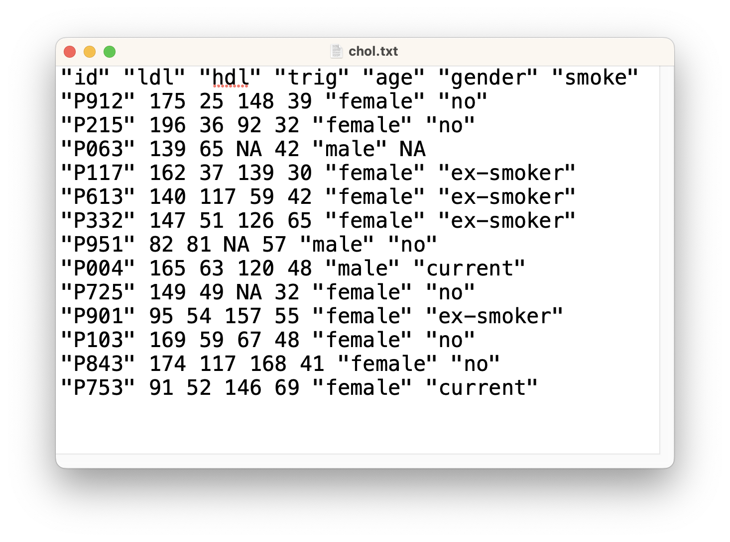
For example, "chol.txt" is shown in Figure 3.1. This is a data set from an observational experiment measuring the cholesterol levels of patients and their smoking status. The variables included are:
"id": a unique code identifying each patient in the experiment."ldl": a measure of each patient's low-density lipoprotein (LDL) cholesterol level."hdl": a measure of each patient's high-density lipoprotein (HDL) cholesterol level."trig": a measure of the triglycerides levels in each patient's blood."age": the patient's age in years."gender": the patient's gender (female or male)."smoke": whether a patient is a current-smoker, ex-smoker, or non-smoker.
We can see in Figure 3.1 that "chol.txt" does include column names (i.e header = TRUE) and that each element of the data set is separated with a space (i.e. sep = ""). The missing values in "chol.txt" are already represented by NA (i.e. the symbol for missing values in R), so we don't need to include na.strings =.

Figure 3.1: Screenshot of chol.txt file
In order to read the file chol.txt into R we can use the following code.
Note that we have left out sep = "" because this is the default value of the argument so it is not required to type it in the function read.table().
It is good practise to compare the object you've just saved in the Environment tab with the contents of the original data file to make sure everything is as you expect. This will highlight any discrepancies and allow you to check whether additional arguments are required to fix them e.g. na.strings = or header =.
3.3 read.csv()
Another common file type that data may be stored in are '.csv' files. If data has been input into Microsoft Excel, it will often be exported as a '.csv' file, so we see these a lot. In order to read '.csv' files into R, we use the function read.csv(). This takes very similar arguments to read.table(), including:
file =: this is the full name of the '.csv' file in quotation marks, provided it is saved in the folder you have set as your working directory.header =: by default this takes the valueTRUE, so column names are automatically included for '.csv' files.sep =: the default separator character issep = ",".na.strings =: the default for denoting missing values in the original '.csv' file is set to"NA".dec =: the default decimal point is set to".".
Again, the only necessary argument in read.csv() is file =.
Read the file "edu.csv" into R and save it as a data frame called education.
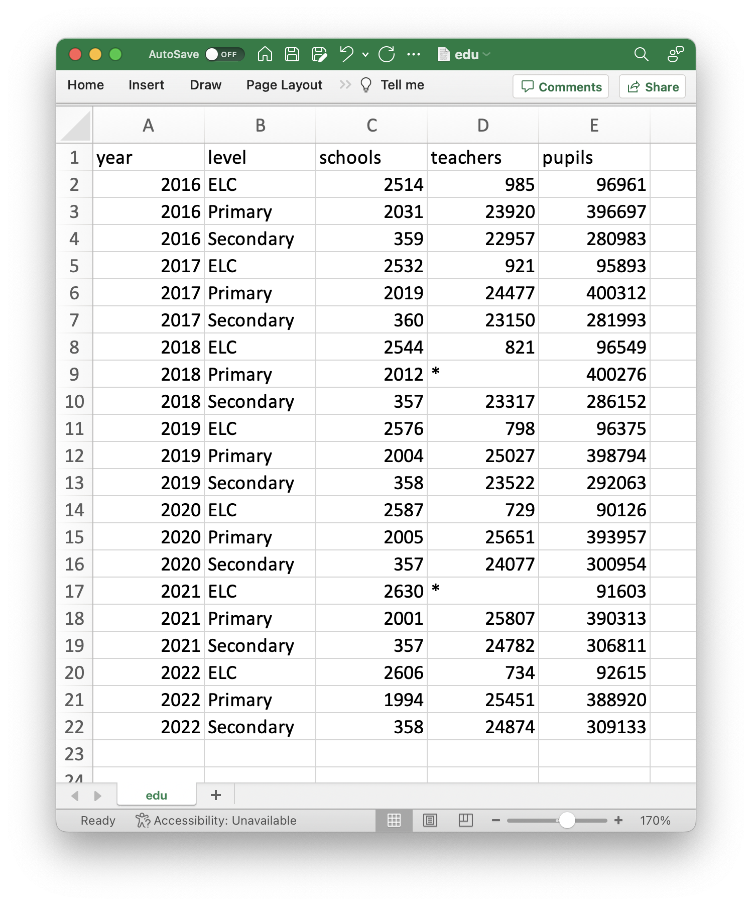
This is a data set containing information on the total numbers of pupils and teachers in schools of different education levels in Scotland. The variables included are:
"year": the year measurements were taken in (2016-2022)."level": the level of education measurements were taken from ("ELC", "Primary" or "Secondary")."schools": the total number of schools across Scotland in the given year/level combination."teachers": the total number of teachers employed in all the schools in the given year/level combination."pupils": the total number of pupils attending all the schools in the given year/level combination.
If you were to look at the original file "edu.csv", you would see something similar to Figure 3.2. Here, we can see that there are column headings and that there are two missing values denoted by "*".

Figure 3.2: Screenshot of edu.csv file
In order to read "edu.csv" into R, we can use the following code.
The use of the functions read.table() and read.csv() is detailed in Section 1.10.1 Using read.table() of Probability and Statistics with R.
There are several other file types that data can be stored in, and numerous ways to read data sets into R. If you are curious about other ways to do this, refer to 1.10 Reading and Saving Data in R in Probability and Statistics with R.